Implementation

Overview

With our Photonic Neural Network Simulator, our aim is to provide an easy-to-use and versatile interface to simulate the time dynamics of excitable neurons and networks of these neurons.

The primary building blocks of our implementation are:

• a neuron class: this class defines an object that takes a time-varying input \(x(t)\) , and emits a time-varying output \(y(t)\).This class contains attributes that allow one to specify the type of model to be solved, the ODE solver to be used (currently support Euler and RK4), the size of the time-step \(dt\) and so on. The neuron class also contains functions that allow us to find the zero-input steady-state of the neuron, as well as stepping the neuron’s history forward in time.
• a network class: this class defines a network formed by connecting neurons. A network is specified by a list of neuron objects. The connections between external inputs to the network and the neurons in the network as well as the connections among the neurons themselves are specified by two adjacency matrices. One matrix specifies the weights of the edges in the graph. The weights control to what extent signals are amplified or attenuated as they propagate. Another matrix specifies time delays from one node to another. The following section describes how to define these connections.
• a models.py: this file contains various neuron models, corresponding to different physical implementations of excitable neurons. Currently support three kinds of Yamada models, the Fitz-Hugh-Nagumo model, and an identity (input = output) model.
• a test.py: this file contains test units to verify the above code is working. Testing is done automatically with Tavis, but can also be run manually.

Usage Demonstration Notebook

In this notebook we demonstrate the usage of our neuron and network classes, calculating and visualizing the dynamics of a single neuron and a simple network. Further examples can be seen in Neuron_plots.ipynb and Network_plots.ipynb in the project github. The preamble to set up this notebook is below, note that Network and Neuron are imported.

import numpy as np
import scipy as sp
import matplotlib.pyplot as plt
from neuron import Neuron
from network import Network
from IPython.display import HTML

Usage of Neuron Class

We first study the dynamics of the “Yamada” Laser neuron model, which describes a two section laser containing a gain region and a saturable absorber. Input optical signals stimulate a photodiode, which controls the current into the gain region. The equations of motion are:

Where \(I\) is the dimensionless laser intensity, and \(G\) and \(Q\) are the inversions of the gain and saturable absorbing media. \(i_{in}\) sufficient to produce \(G+Q>1\) results in a sharp laser pulse and the system then refracts. For excitability, we require \(\gamma\ll\kappa\): the field intensity is our fast “state” variable and the inversions are slow “recovery” variables, like the membrane potential and ion permeability respectively in biological neurons.

We begin by choosing our model parameters, contained in the dict Y1mpars below, and then the parameters for the neuron itself, Y1params. The equations of motion above are contained in models.Yamada_1, so we specify this, as well as mpars and the timestep dt. It is important that we initialize our neuron in its steady state, so we use the neuron member function steady_state to compute the steady state for our specific choice of model parameters. To be successful, this requires an initial guess of the steady state, which is y1_steady_est. We then update the full set of parameters Y1params for the Neuron object we will be creating.

#Create a basic Yamada Neuron
#these are the model parameters
Y1mpars={"a": 2, "A": 6.5, "B":-6., "gamma1": 1,
         "gamma2": 1, "kappa": 50, "beta": 5e-1 }

#neuron parameters
Y1params={"model" : "Yamada_1","dt": 1e-2, 'mpar': Y1mpars}

#quick estimate of steady state
y1_steady_est=[Y1mpars['beta']/Y1mpars['kappa'],
               Y1mpars['A'],Y1mpars['B'] ]

 #compute true steady state
y1_steady=Neuron(Y1params).steady_state(y1_steady_est)
#add steady state to model parameters
Y1params["y0"]=y1_steady
#now just use Y1params to initialize neurons

We now proceed to initialize a Neuron with neuron_object=Neuron(neuron_parameters). We then construct an input signal x1 which is a series of Gaussian inputs, the first of which is below threshold and will not cause the neuron to spike, and the last is very noisy but will. The Neuron dynamics in response to this signal are then computed with output=neuron_object.solve(input)

#initialize neuron
Y1Neuron=Neuron(Y1params)

#create time signal
t1_end=9. #final time point
N1=int(np.ceil(t1_end/Y1Neuron.dt)) #this many points
time1=np.linspace(0.,(N1-1)*Y1Neuron.dt, num=N1 )

#normalized guassian for constructing input signals
Gaussian_pulse= lambda x, mu, sig: np.exp(-np.power(x - mu, 2.)
    / (2 * np.power(sig, 2.)))/(np.sqrt(2*np.pi)*sig)
#create input signal x1
x1=np.zeros(N1)
x1+=0.2*Gaussian_pulse(time1, 0.1, 1.e-2)
x1+=0.5*Gaussian_pulse(time1, 2., 1.e-2)
x1+=0.5*Gaussian_pulse(time1, 6.5, 5.e-2)*np.random.normal(1,1,N1)

#solve
y_out1=Y1Neuron.solve(x1)

These results are visualized with figure=neuron_object.visualize_plot(input, output, time, steady_state).

The upper axis contains the input current to the neuron, and the lower is the resultant dynamics. The light intensity is the left axis in blue and the gain and absorber inversions are in red and green on the right axis. The steady states are also indicated with dashed lines. Note that a spike is not seen for the initial Gaussian input pulse, as its area is below threshold. The second and third pulses have the same area and thus produce nearly identical responses, even though the later is quite noisy. The refractory period can also be seen as the large time it takes for the inversion variables to recover after each spike.

fig1=Y1Neuron.visualize_plot(x1, y_out1, time1, y1_steady)
#can use returned figure object to customize plot, as below
fig1.set_size_inches(10, 8, forward=True)

Usage of Network Class

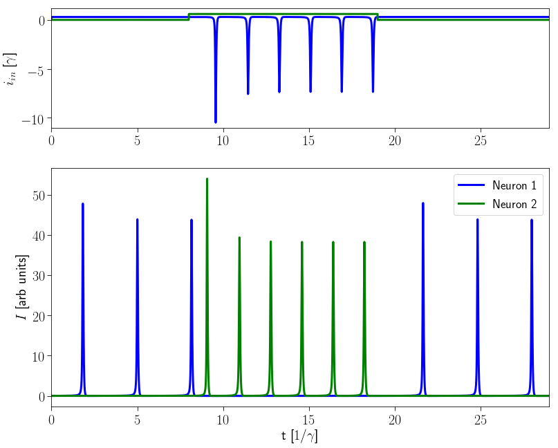
We next consider an inhibitory network of two neurons, each with their own input channel. Neuron 2 is inhibitively connected to neuron 1: when it fires it prevents Neuron 1 from firing. These simple networks often govern reflex behaviors such as the knee-jerk: When the knee is tapped, the patellar sensory neuron fires, this inhibits a motor neuron controlling the flexor hamstring muscle, causing it to relax and allowing your leg to kick out.

We first construct a list of 2 identical neurons (neurons=[Neuron(Y1params), Neuron(Y1params)]) with the same parameters as the original neuron studied above. We then define our weight and delay matrices (weights=np.array(...), delays=np.array(...)), and use these to create a network: network=Network(neurons, weights, delays). The structure of the weight and delay matrices are discussed further in the “Defining Network Connections” section of this documentation.

# Inhibitory 2 input 2 neuron network
#list of 2 neurons
neurons=[Neuron(Y1params), Neuron(Y1params)]
#neuron 1 receieves input,feeds to neuron 2
weights=np.array([[1.,0.,0., -0.2],[0.,1.,0., 0.]])
#Delay on signal from neuron 1 to neuron 2
delays=np.array([[0., 0.5], [0., 0.]])

#create network
network2=Network(neurons, weights, delays, dt=0.001)

Since our network accepts two inputs, our input signal is now a 2-D numpy array, with each column corresponding to a different input channel. For a given set of input signals, the network dynamics are calculated with output=network.network_solve(input). The Network class also has a member function which computes the total time-dependent input (sum of internal and external) to each neuron, to better understand and visualize the network dynamics, this is done via total_input=network.network_inputs(output, input). Note that the external inputs are the second argument.

t2_end=29.
N2=int(np.ceil(t2_end/network2.dt)) #this many points
time2=np.linspace(0.,(N2-1)*network2.dt, num=N2 )

in2=np.zeros([N2, 2])
#scale with gamma1 so drive in units of A
#drive neuron 1 continuously just above threshold
in2[:, 0]+=(0.3)*np.heaviside(time2, 0.5)
#Drive neuron 2 for a short period then turn off
in2[:, 1]+=(0.6)*np.heaviside(time2-8., 0.5)
in2[:, 1]+=(-0.6)*np.heaviside(time2-19., 0.5)

#solve network
output2=network2.network_solve(in2)
#compute inputs
input2=network2.network_inputs(output2, in2)

The resultant dynamics are plotted below via:figure=network_object.visualize_plot(input, output, time).

The upper axes contains the total (weighted, delayed, and summed) input to each neuron as a function of time, and the lower axes the state of each neuron (dimensionless laser intensity). Note that once neuron 2 starts firing, neuron 1 stops because neuron 2 inputs a large negative spike to neuron 1.

#use visualize_plot quickly plot of the network dynamics
fig2=network2.visualize_plot(input2, output2, time2)
fig2.set_size_inches(10, 8, forward=True)

Below is a visualization of the same dynamics as an animated graph, generated using the member function visualize animation. To see the resultant animation, We need to call HTML(animation.to_`.to_html5_video()) where HTML was imported from IPython.display

Each neuron is depicted as a node of the network which brightens when it fires. The connectivity between network elements and their relative strengths are also indicated.

%%capture
an2 = network2.visualize_animation(inputs=in2, outputs=output2);
#create animation
#capture is to supress output,
#remove to generate a static image of the network

#view animation
HTML(an2.to_html5_video())
#note that this HTML call can be time-consuming

Defining network connections

A network can be thought of as a system of inputs and outputs.

To construct your W matrix, consider the examples in the following images.

Simple network

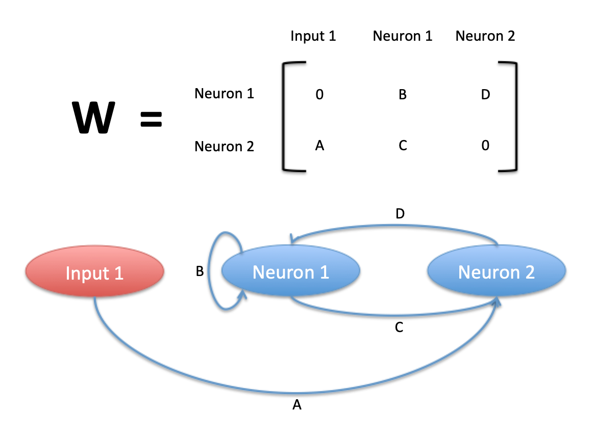
Complicated network

Multi-input network

Each row corresponds to a neuron. Each column corresponds to an input source, with the raw inputs coming first and the neurons coming second. The element of W in row i and column j should be interpreted as “neuron i gets its input from input-source j”.

The time delay matrix is simpler. In a similar way, the element of T in row i and column j should be interpreted as “neuron i gets its input from neuron j”.

Time delay matrix format